Ultrasonic Ranging
Using the latest SensEdu Shield on an Arduino Giga R1 platform, we want to get the distance measurements for all 4 MEMS microphones. In this project, we use SensEdu Library and DMA approach for fast and efficient data acquisition. This can represent a prerequisitie for other projects for further processing the distance measurements. The data from the microphones is processed and sent via Serial Communication on a PC.
The project is divided into 2 main parts:
- Arduino GIGA R1 WiFi with SensEdu Shield: Data acquisition and sending the measurements data
- PC with MATLAB: Starting the data acquisition and receiving the measurements data
Serial Communication
The communication is done using a Half Duplex method and UART communication protocol - each sender and receiver can transmit the data but not at the same time. This is needed since the data acqusition is started only after the PC (sender) sends the starting signal to the board. After the starting signal, data acquisition and data sending is performed for a predefined amount of time.
Data Acquisition and Sending the Data
The following data acquisition flow chart explains the algorithm.
Since the microcontroller is ecquiped with three ADCs and we use four microphones, we use two ADCs - ADC1 and ADC2 accessing through two channels all four microphones. The ADC sampling rate is set to 250 kHz.
The exact sampling rate is very important for exact measurement acquisition. Make sure it matches throughout the code.
About the Sampling Rate
In this project, the ADC sampling rate is set to 250 kHz.
How to change ADC Sampling Rate?
Changing the ADC sampling rate correctly requires the following steps:
- In .ino script - set “.sampling_freq” field of SensEdu_ADC_Settings structure
- In .ino script - set “ACTUAL_SAMPLING_RATE” macro to the same value
- In “generateDAC.m” - set “fs” variable to match the wanted sampling frequency and generate a new LUT
- Copy the new LUT to the “SineLUT.h” file
Currently, the library does not support different sampling rates for different ADCs since all the ADCs use the same timer.
As for the DAC sampling rate, it is caluclated as frequency of the wave that is sent - in our case 32 kHz sine wave multiplied by the number of samples that the wave has for one cycle.
To generate the measurements, first burst sine signal with 32 kHz frequency is sent through DAC1. The sine wave is stored in a lookup table (LUT) as an uint16_t array.
After the burst is sent, ADC starts to collect the data microphones are receiving. The raw data is represented with 16bit values corresponding to the changes in pressure received by microphones.
How is the distance computed
The main difference between the audible sound and ultrasound is the frequency range. Other characteristics are the same. Therefore, we know that the sound travels through the air with constant speed of about 343 m/s. Since the speed is constant, the distance can be calculated using the simple formula for constant motion:
\[\begin{equation} v = \frac{d}{t} \label{eq:speed} \end{equation}\]Therefore, the time is what we need to compute the distance. The time is computed as a time-of-flight (TOF) of the reflected DAC signal from the object. To compute the TOF, the cross-correlation method is used. Cross-correlation method essentially compares two signals and detects the point at which they have the most similarity. In this case, the cross-correlation is performed between the output wave of the DAC and input wave of the ADC.
For correct cross-correlation, DAC output signal has to have the same sampling rate as the ADC signal. Therefore, this signal is additionally computed using the provided MATLAB script “dac_wave_gen.m”. Make sure to adjust the sampling rate in the script to the real sampling rate of the ADC previously computed!
There are two intersteps before the cross-correlation is performed:
Rescaling the ADC signal
The ADC signal has values in range [0, 65535]. Therefore, we first rescale the signal to have the range [-1, 1] with each sample being a 4-byte float value using the “rescale_adc_wave” function.
Because of the way multi-channel ADC signals are stored in memory using SensEdu library, the channel number has to be passed to the function.
Filtering the rescaled signal
Since we are working with microphones with frequency range between 20 Hz and 100 kHz, they are very sensitive to audible sound as well. This is undesired in our case because we want to have a signal that is around 32 kHz in order to get good results. Therefore, a Finite Impulse Response (FIR) bandpass filter is applied to the previously resacaled ADC signal using the “filter_32kHz_wave” function.
Finally, the cross-correlation method is performed on the filtered signal and ouput signal. The result of the cross-correlation is number of lag samples between the two signals. Then, the distance is computed as:
\[\begin{equation} d = \frac{(lag\_samples \cdot sample\_time)}{sampling\_rate \cdot 2} \end{equation}\]Two modes are possible for sending the data depending on the value of preprocessor macro “XCORR_DEBUG”. Setting this value to true sends raw-, rescaled-, and filtered data with distance measurements to the PC. Otherwise, only the distance measurements will be sent to the PC.
For faster measurements, cross-correlation is performed directly on the microcontroller. However, if the time-efficiency is not a requirement, setting preprocessor macro “LOCAL_XCORR” to false will directly send raw ADC data to the PC.
Receiving the Data
Data is received on the PC using MATLAB script plot_microphones_data.m. The function read_mcu_xcorr.m reads the distance data, and the function read_mcu_xcorr_details.m reads raw-, rescaled-, and filtered data.
Since we are using serial communication, the data is received one bit at a time. To start receiving the data from the microcontroller, the PC initiates the communication by sending the starting byte.
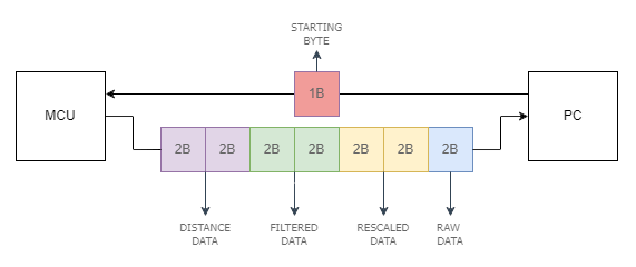
This diagram depicts one iteration of PC receiving the data. This continues for number of iterations that are specified in the MATLAB script. Then, the data is plotted for visualization.
Make sure that PLOT_DETAILED_DATA in MATLAB matches the value of XCORR_DETAILS, as well as to set DATA_LENGTH in MATLAB to be the same as STORE_BUF_SIZE macro. Make sure to choose the correct ARDUINO_PORT to match the real one.