FMCW Radar
This project is currently in its initial development phase and is subject to significant changes, updates, and improvements. The project enables a rudimentary implementation of an FMCW radar and requires two Arduino boards with SensEdu Shields.
The FMCW Radar Project utilizes the SensEdu Shield to perform distance measurements using FMCW radar techniques.
FMCW radars are widely used for short range applications like automotive or drone ranging. These radars have the advantage of providing good spatial resolution while being simple to implement.
Table of contents
FMCW Radar Principle
This chapter explains the fundamentals of FMCW radars in order to better understand their magic. For more in-depth information, I would recommend Marshall Bruner’s YouTube channel — his channel is a gem on the subject! The animated graphs on this doc have been created with the Manim Community python library and are greatly inspired by Marshall Bruner’s code.
Chirp Signal
FMCW radars involves the continuous transmission and reception of a frequency modulated signal also known as chirp. We will call the transmitted signal \(T_x\) and we are using a sawtooth modulation. The sawtooth modulation linearly sweeps a bandwidth \(B\) over the chirp period \(T_c\).
The transmitted signal is reflected from a static object and received by the radar. The received signal is called \(R_x\). Below is a representation of \(T_x\) and \(R_x\)’s amplitude and frequency over time :
\(T_x\) and \(R_x\)’s Amplitude and Frequency as a Function of Time
As we see, \(R_x\) is exactly the same signal as \(T_x\) but delayed by \(t_0\), the time of flight (TOF). We can intuitively establish a relationship between \(t_0\) and the distance to the object :
where
- \(c = 343 \, \text{m} \cdot \text{s}^{-1}\) the speed of sound in air \((T = 293 \, K)\)
- \(d\) is the distance to the object \(\text{(m)}\)
Distance
Where pulse radars measure time and TOF to evaluate distance, FMCW radars measure frequencies! The TOF \(t_0\) cannot be estimated directly since we are sending waves continuously but we have another valuable information : The beat frequency \(f_b\).
The beat frequency is defined as the frequency equal to the difference between two sinusoids. \(f_b\) appears in the figure below :
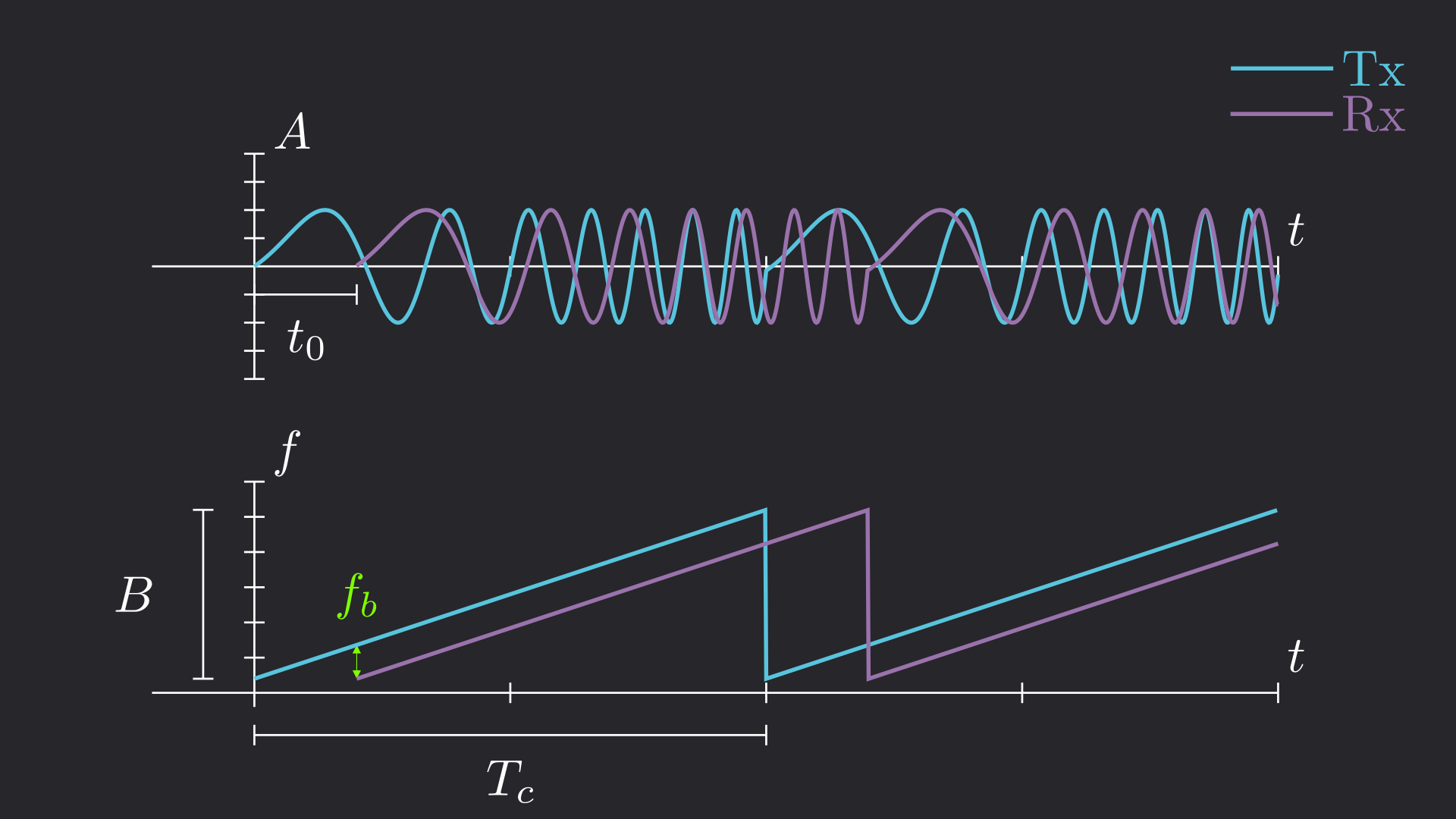
The Beat Frequency \(f_b\) appears due to the slight delay between \(T_x\) and \(R_x\)
The geometrical approach is the simplest way to understand how to derive the distance from \(f_b\). Let’s define the slope of the chirp \(s\) being \(s=\frac{B}{T_c}\). Using the last figure and Eq (1) we now have the following relationship :
Thus, the distance can easily be derived :
We know how to compute the distance, that’s great! But how do we extract \(f_b\) …
Beat frequency
To extract the beat frequency we need to mix the \(T_x\) and \(R_x\). Mixing two signals is essentially multiplying them but it enables us to subtract in the frequency domain.
If we freeze \(T_x\) and \(R_x\) at a given time, they’re basically two sinusoids at different frequencies. Let’s define \(f_T\) and \(f_R\) the instantaneous frequencies of our two signals where \(f_T>f_R\) (the phase of the signals is not relevant here). We also define \(y_{mix}\) the mixed signal.
At a given time, \(y_{mix}\) is expressed as
The mixing operation produces a signal which is the sum of two sinusoids :
- One at the frequency \(f_{T}-f_{R}\)
- One at the frequency \(f_{T}+f_{R}\)
The high frequency component HF at \(f_{T}+f_{R}\) can easily be removed with a low pass filter. The remaining signal is a simple sinudoid at the beat frequency \(f_b=f_{T}-f_{R}\). Below is a representation of the mixing signal operation :
\(y_{mix}\) is the product of \(T_x\) and \(R_x\)
Distance Resolution & Max Range
Distance resolution and max range are two critical parameters regarding radar performance. Distance resolution defines the smallest distance between two objects that the radar can detect as distinct targets. The distance resolution \(\Delta d\) is defined by
where
-
\(c\) is the speed of sound \(\text{(m} \cdot \text{s}^{-1})\)
-
\(B\) is the bandwidth of the chirp \(\text{(Hz)}\)
Distance resolution is only dependent on the radar’s bandwidth !
For ultrasonic FMCW radars, the maximum range \(d_{max}\) is heavily limited by \(T_c\). The maximum range \(d_{max}\) is defined by
where
-
\(c\) is the speed of sound \(\text{(m} \cdot \text{s}^{-1})\)
-
\(T_c\) is the period of the chirp \(\text{(s)}\)
For ultrasonic FMCW radars, the max range bottleneck is \(T_c\). For regular FMCW radars, it’s usually the ADC sampling frequency.
Radar Design
The following block diagram illustrates the architecture of the FMCW radar :
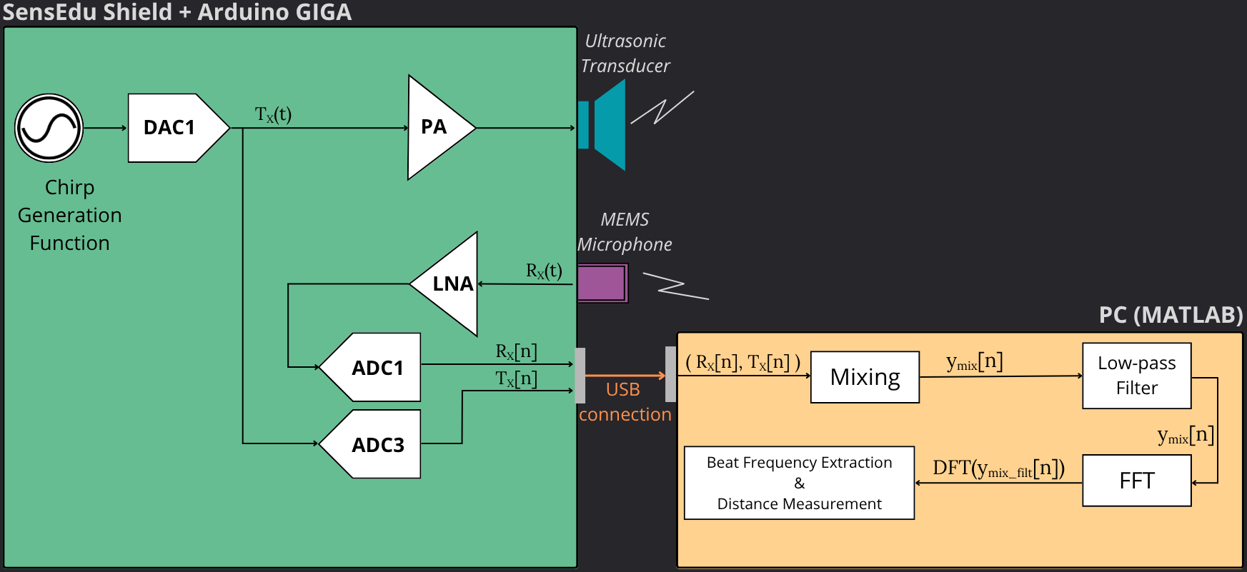
FMCW Radar Block Diagram
The chirp signal Tx is generated and converted to an analog signal with the DAC. Tx is then doubled and follows 2 paths :
- Tx is amplified and sent to the ultrasonic transducer
- Tx is sent to ADC3 by using a jump wire between the DAC pin and the receiver ADC3 pin (A8).
The MEMS microphone receives a signal Rx which is amplified with a low noise amplifier (LNA) and goes through ADC1. The digital Tx and Rx signals are both sent to MATLAB.
The following signal processing is performed in MATLAB to measure the distance between the two shields :
- Compute mixing operation between Tx and Rx
- Compute FFT of mixed signal \(y_{mix}\)
- Low-pass filter \(y_{mix}\)
- Extract beat frequency and compute distance
Code Implementation
Make sure to wire the DAC output to ADC3 (analog pin A8).
Sending the ADC data and receiving in MATLAB
- ADC3 receives the DAC data
- ADC1 receives the microphone #3 data
A size header adc_byte_length is sent to MATLAB to indicate the size of each ADC frame in bytes. Since ADCs are 16-bit, each data is coded with 2 bytes. The data from both ADCs is sent to MATLAB using the serial_send_array function.
// Send ADC data (16-bit values, continuously)
    uint32_t adc_byte_length = mic_data_size * 2; // ADC data size in bytes
    Serial.write((uint8_t*)&adc_byte_length, sizeof(adc_byte_length));  // Send size header
    serial_send_array((const uint8_t*)adc_dac_data, adc_byte_length);       // Transmit ADC3 data
    serial_send_array((const uint8_t*)adc_mic_data, adc_byte_length);       // Transmit ADC1 data (Mic3 data)
An important variable is mic_data_size which must be a multiple of 32 because serial_send_array sends data by chunks of 32-bytes. mic_data_size will also define the amount of samples used for the plots in MATLAB.
The bigger the value of mic_data_size, the more latency when you run the MATLAB distance measurement script but the more signal will be displayed on the plots.
// Retrieve size header for ADC data
    adc_byte_length = read_total_length(arduino);      // Total length of ADC data in bytes
    ADC_DATA_LENGTH = adc_byte_length / 2;             // Total number of ADC samples

    // Retrieve DAC to ADC data
    adc3_data = read_data(arduino, ADC_DATA_LENGTH);

    // Retrieve Mic ADC data
    adc1_data = read_data(arduino, ADC_DATA_LENGTH);
Data processing in MATLAB & Distance computation
After sending the data to MATLAB, the data can be processed and the distance is eventually computed. It is worth noting that a high-pass FIR filter has also been applied to the mixed signal in MATLAB. This is to attenuate low frequencies (15 Hz to 46 Hz) in the spectrum coming from the transducer’s signal directly received by the microphone. These frequencies don’t correspond to an object’s reflection and thus need to be mitigated. This is important to mitigate the right amount of reflections
Here are the different steps in order to compute the distance in MATLAB.
Step 1 : High pass filter Tx (adc3_data) and Rx (adc1_data) to clean up the signals
    adc3_data_filt = highpass(adc3_data, 30000, SAMPLING_RATE);
    adc1_data_filt = highpass(adc1_data, 30000, SAMPLING_RATE);
Step 2 : Mix Tx and Rx using sample-by-sample multiplication
mixed_signal = adc3_data_filt .* adc1_data_filt;
Step 3 : Low-pass filter the mixed signal at 5 kHz to remove the unwanted high frequency component
mixed_signal_filt = lowpass(mixed_signal, 5000, SAMPLING_RATE);
Step 4 : Compute the power spectrum density (PSD) of the mixed filtered signal
[p_mix_filt, f_mix_filt] = pspectrum(mixed_signal_filt, SAMPLING_RATE);
Step 5 : Extract the beat frequency from the PSD of the mixed filtered signal
[p_fbeat,fbeat] = findpeaks(p_mix_filt,f_mix_filt,NPeaks=1,SortStr="descend");
Step 6 : Compute the distance
d = (fbeat * Tc * c) / (2*(f_end - f_start));
Make sure the parameters in MATLAB match the parameters of the chirp you are sending (f_start, f_end, Tc, etc…).
After running the MATLAB code, you should see the following display. This example is with an object placed at 50 cm from the board and using the following radar parameters :
- f_start = 30.5 kHz
- f_end = 35.5 kHz
- Tc = 40 ms
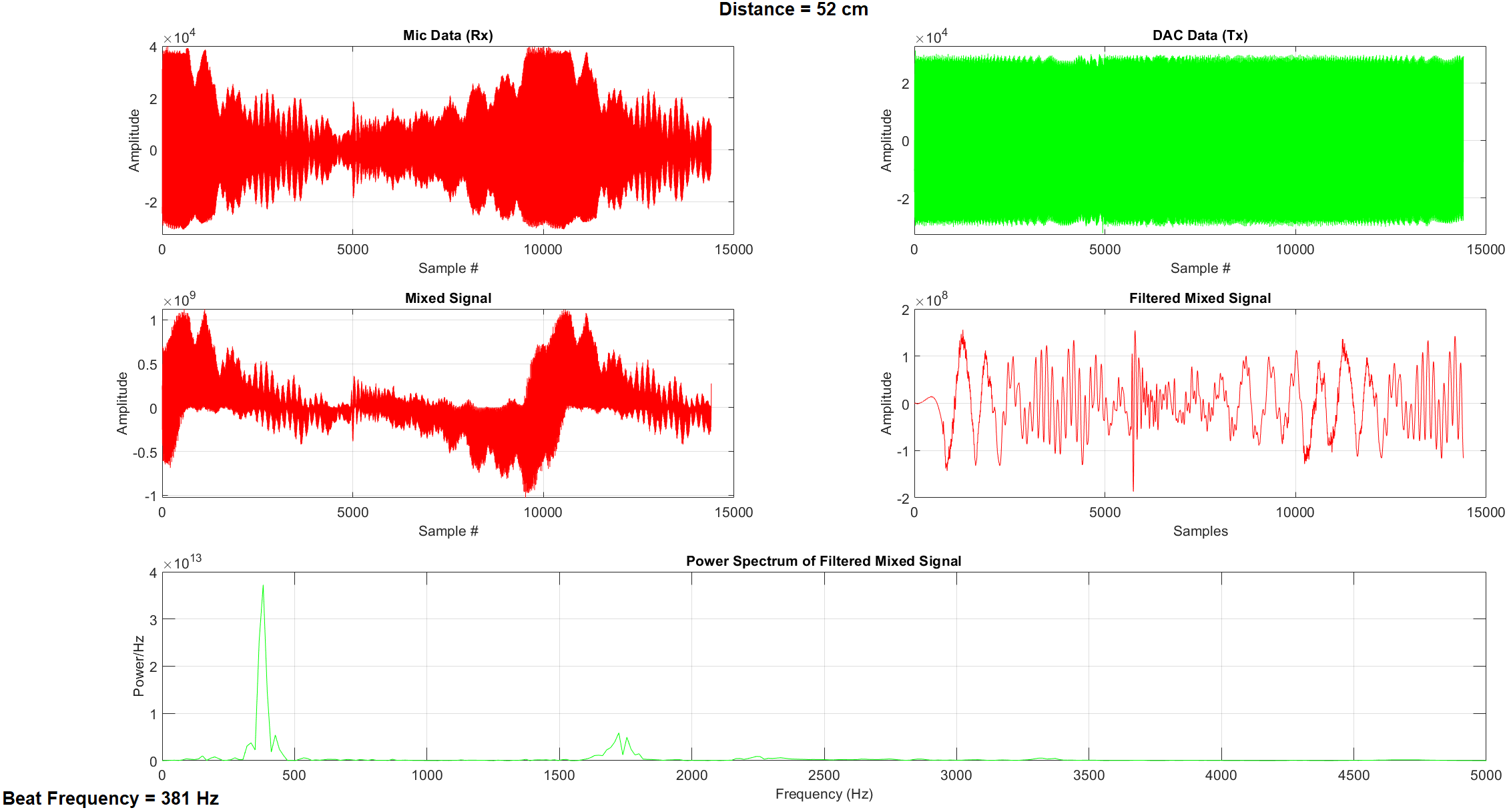
Measurement display in MATLAB