EMG BioInputs

---

• Introduction
• Biological Background
• Recording Action Potentials
• Hardware Setup
  • Electrodes Connectivity
  • Amplifier Circuit
  • Data Acquisition
  • Data Transfer
• Signal Processing
  • Problematic ADC Readings
  • The Buffer
  • FIR Filter
  • Rectification
  • Envelope
  • Decision Block
  • Press problems
  • Capacitive input
• Testing
• Showcase
• Possible improvements
• Appendix: data recordings for improvements
• Good study on perfect high pass value
• Good Resources:
• Sources:

Introduction

Electromyography (EMG) is a widely-used technique for recording and analyzing electrical activities generated by skeletal muscles.

EMG is appealing due to its simplicity when detecting basic movements, such as a biceps contraction. For such projects, advanced hardware or complex signal processing is often unnecessary. This makes EMG an accessible tool for beginners as an introduction into biomedical engineering projects. Furthermore, the foundational concepts learned through EMG can be extended to related fields, including Electrocardiography (ECG), Electrooculography (EOG), Electroencephalography (EEG), and others.

In SensEdu, we demonstrate how basic biceps contraction can be used to simulate keyboard press logic, with latency of ~100–200ms. We use the most basic circuit design combined with signal processing in MATLAB.

This page will guide you step-by-step through the required setup and knowledge to create a simple yet effective demonstration of a typical biomedical engineering project.

Biological Background

First, we need to establish an understanding of what we are trying to measure.

Highly recommended watching the video Neuromuscular Junction by Byte Size Med.

The most important structure that we need to focus on is the Neuromuscular Junction (NMJ). This is a specialized synapse that acts as a communication bridge between motor neurons and skeletal muscle fibers. The NMJ plays a fundamental role in converting neural signals into muscle contraction. Let’s break down its working principle step by step.

The process begins with a motor neuron transmitting an electrical signal called an Action Potential. This signal travels along neuron’s axon until it reaches the NMJ. It activates voltage-gated sodium channels, which allow positively charged sodium ions (Na⁺) enter the cell. The influx of sodium causes the cell membrane to become “less negatively charged”, a change known as depolarization.

Continuous depolarization of the cell membrane subsequently activates voltage-gated calcium channels. Calcium ions (Ca²⁺) flow into the cell which triggers little containers with neurotransmitters to fuse with the membrane and release Acetylcholine (ACh).

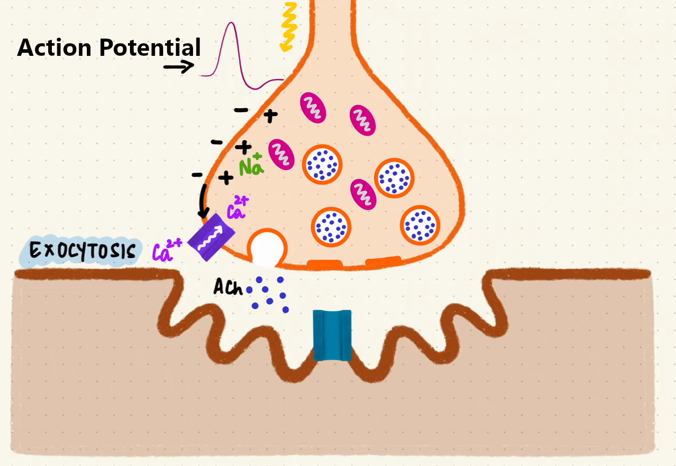
Exocytosis process at the Neuromuscular Junction (source: Byte Size Med)

Acetylcholine travels across the synaptic space and binds to specialized receptors on the muscle cell’s membrane. These receptors, also known as ligand-gated ion channels, respond to the chemical messenger (neurotransmitter) by opening and allowing ions to enter the muscle cell. This process triggers membrane depolarization, causing the resting membrane potential of the muscle cell (normally at around -90mV) to become less negative.

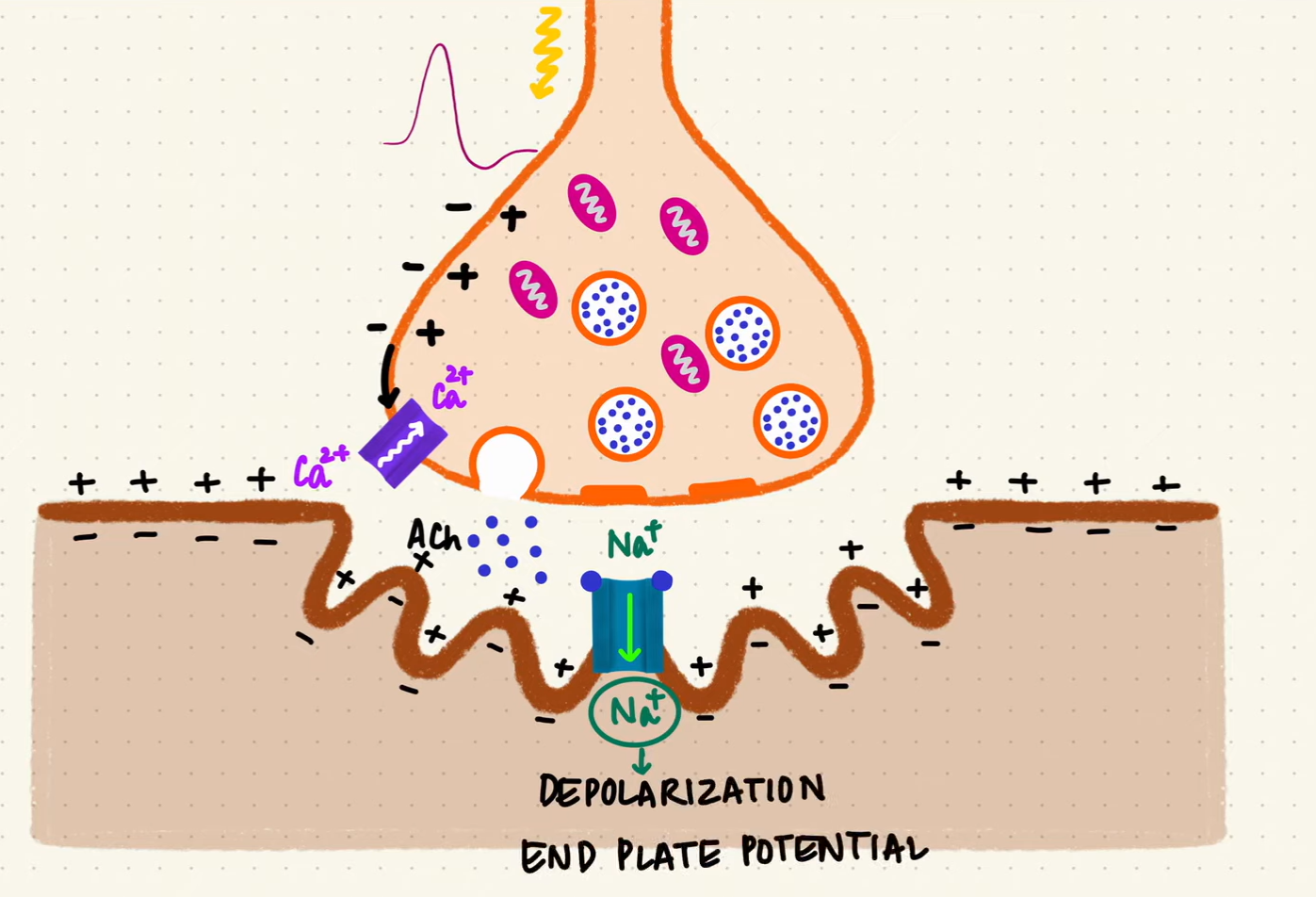
Depolarization caused by the opening of ligand-gated ion channels (source: Byte Size Med)

As more ACh molecules bind to their receptors, the membrane voltage continues to rise. Once it reaches a threshold of approximately -50 mV, voltage-gated sodium channels open, allowing sodium ions (Na⁺) to rush into the muscle cell. This influx of sodium completes the process of membrane depolarization and generates an Action Potential. This electrical signal propagates along the muscle membrane, eventually leading to a muscle contraction.

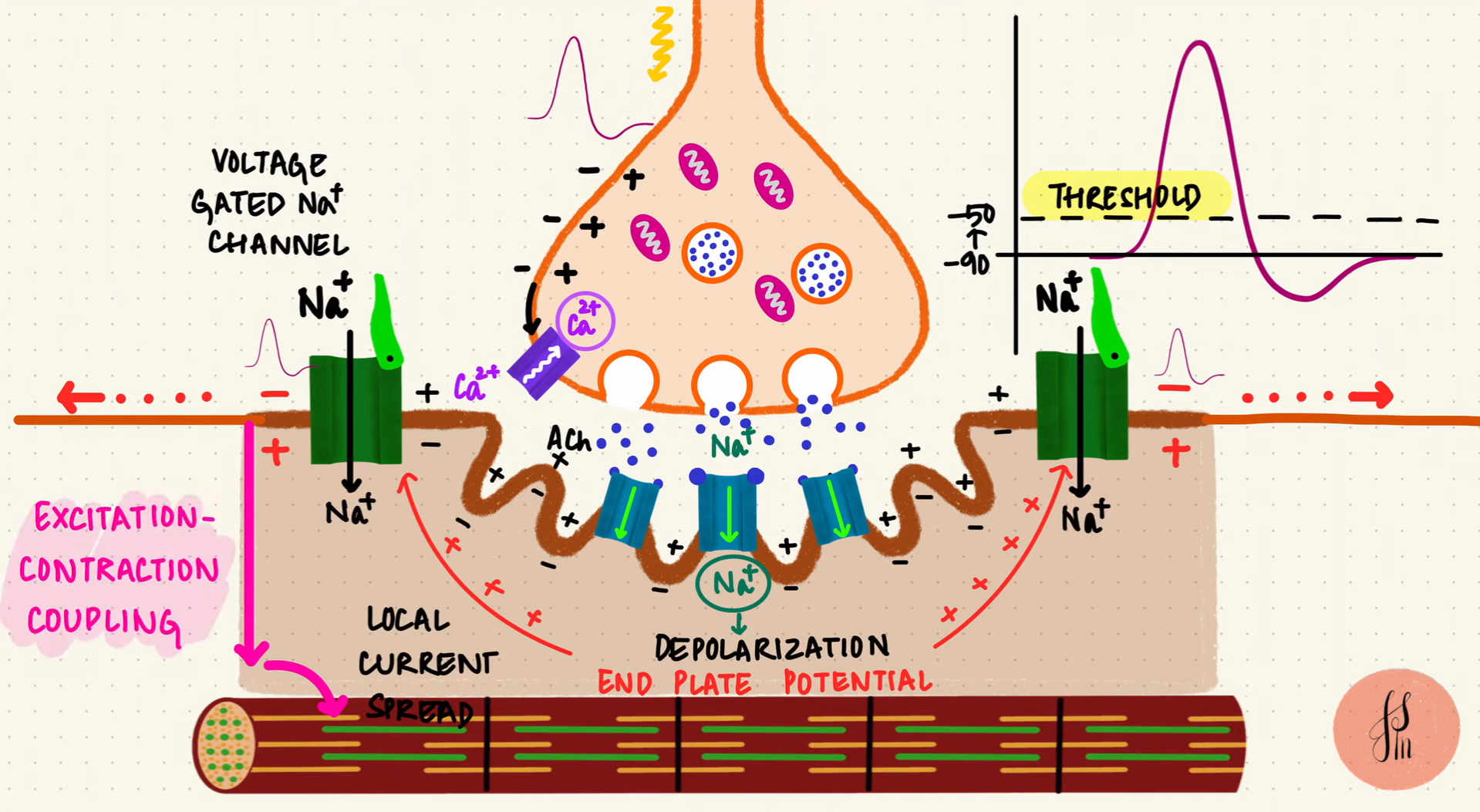
Excitation-Contraction Coupling (source: Byte Size Med)

If you feel overwhelmed by the details, the main takeaway: a neural electrical signal is converted to a chemical signal and then back into electrical signal in the muscle. The sequence Neural Action Potential → Acetylcholine Release → Muscle Action Potential. The muscle action potential then propagates along the muscle cell membrane and ultimately triggers muscle contraction.

The most important point is that this muscle action potential can be measured, providing valuable information about muscle activity.

Recording Action Potentials

Action Potentials can be recorded using different methods:

• Invasive Needle EMG: Inserting electrodes directly into the muscle, enabling highly precise and localized recordings. It is widely used in clinical applications and treatments where precision and measurement quality are critical.
• Non-invasive Surface EMG: Placing electrodes on the skin above the muscle. This approach improves patient comfort and simplifies repeatable studies, making it ideal for educational purposes. However, sEMG has significant precision limitations due to the layers of skin and fat between the electrodes and the muscle. These limitations make it challenging to differentiate the activity of individual muscle fibers and to record signals from small muscles, like ones around the fingers.

In SensEdu we use surface EMG. From now on, whenever we mention EMG or electrodes, we are referring to sEMG and surface electrodes, respectively.

Hardware Setup

This section describes the necessary connections and hardware details required for the proper setup of the EMG BioInputs system and writing the script for MCU. Below is an illustration of the overall system architecture.

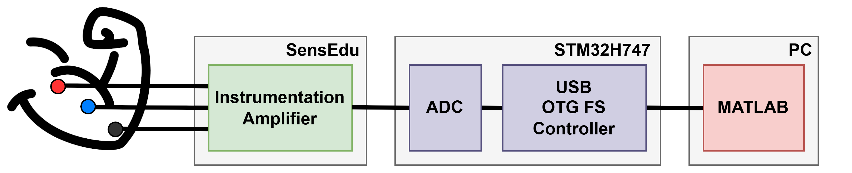
EMG BioInputs System Architecture

Electrodes Connectivity

The system supports up to 4 EMG probes, which can be connected via female 4-Pin 2.54 headers: J9, J11, J12, and J20.

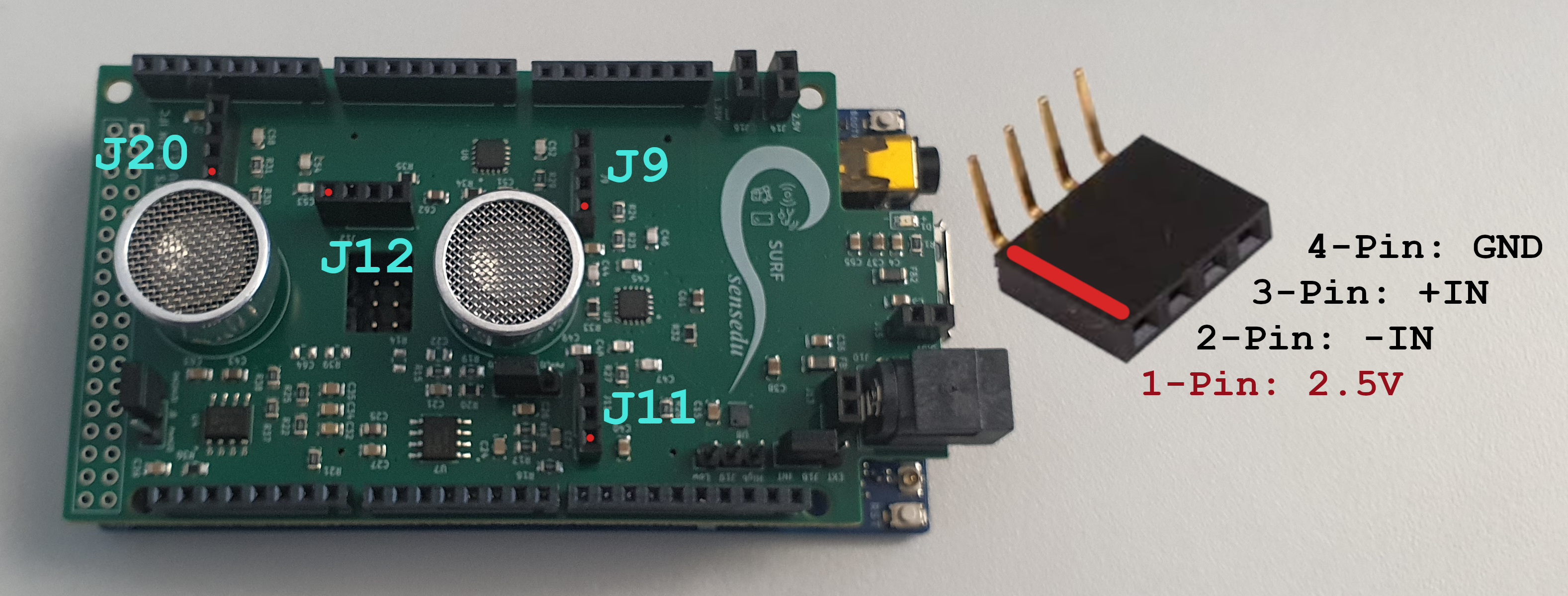
SensEdu input headers (red dots mark the 1st pin)

A typical electrode consists of 3 connectors: Reference, Positive Input, and Negative Input. Below is a table detailing how these connectors correspond to the pins on the headers. Note that the voltage pin (1st pin) on the headers is not used in this connection.

Electrode Connector	Signal	Header Pin
Negative Input	–IN	2nd Pin
Positive Input	+IN	3rd Pin
Reference	GND	4th Pin

Most commercially available electrodes use connectors that are not directly compatible with typical 2.54 headers. For specific chosen electrode you will need a solution how to make this connection possible via soldering, custom adapters, or ready-made solutions.

In our example, we used the following electrodes:

Manufacturer	Product Title	Product Code	Datasheet	Store
SparkFun Electronics	Electrode Pads	12970	link	link
MTG Imiella Medizintechnik	Liquid Gel Disposable Electrodes for ECG (Ø40mm)	S40LG	link	link

These electrodes use a mini-jack connector. To simplify the connection, we designed a simple PCB adapter called MiniJack2Jumper. This adapter is inserted vertically into the SensEdu header, providing a mini-jack socket and eliminating the need for soldering. All PCB source files, including Gerbers and BOM, are available in the directory: /Projects/EMG-BioInputs/pcbs/MiniJack2Jumper. To replicate our setup, you can use archive MiniJack2Jumper/manufacturing/MiniJack2Jumper-Gerber.zip to order the PCB from any cheap Chinese manufacturer. The cost typically ranges from $15–$30 depending on shipping.

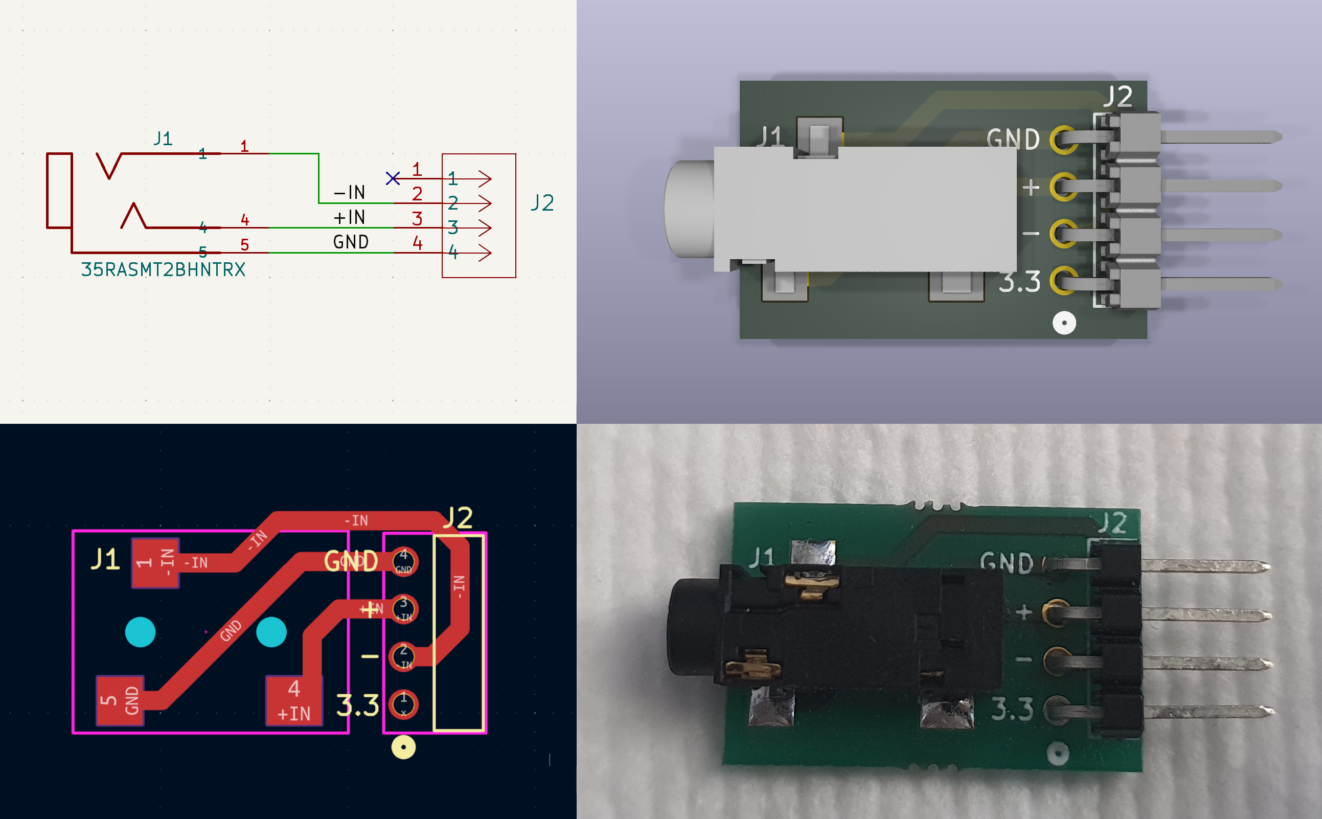
MiniJack2Jumper adapter: Schematics, PCB view, 3D view, and real-life view

After connecting the electrodes using the MiniJack2Jumper adapter, the final setup looks as follows:

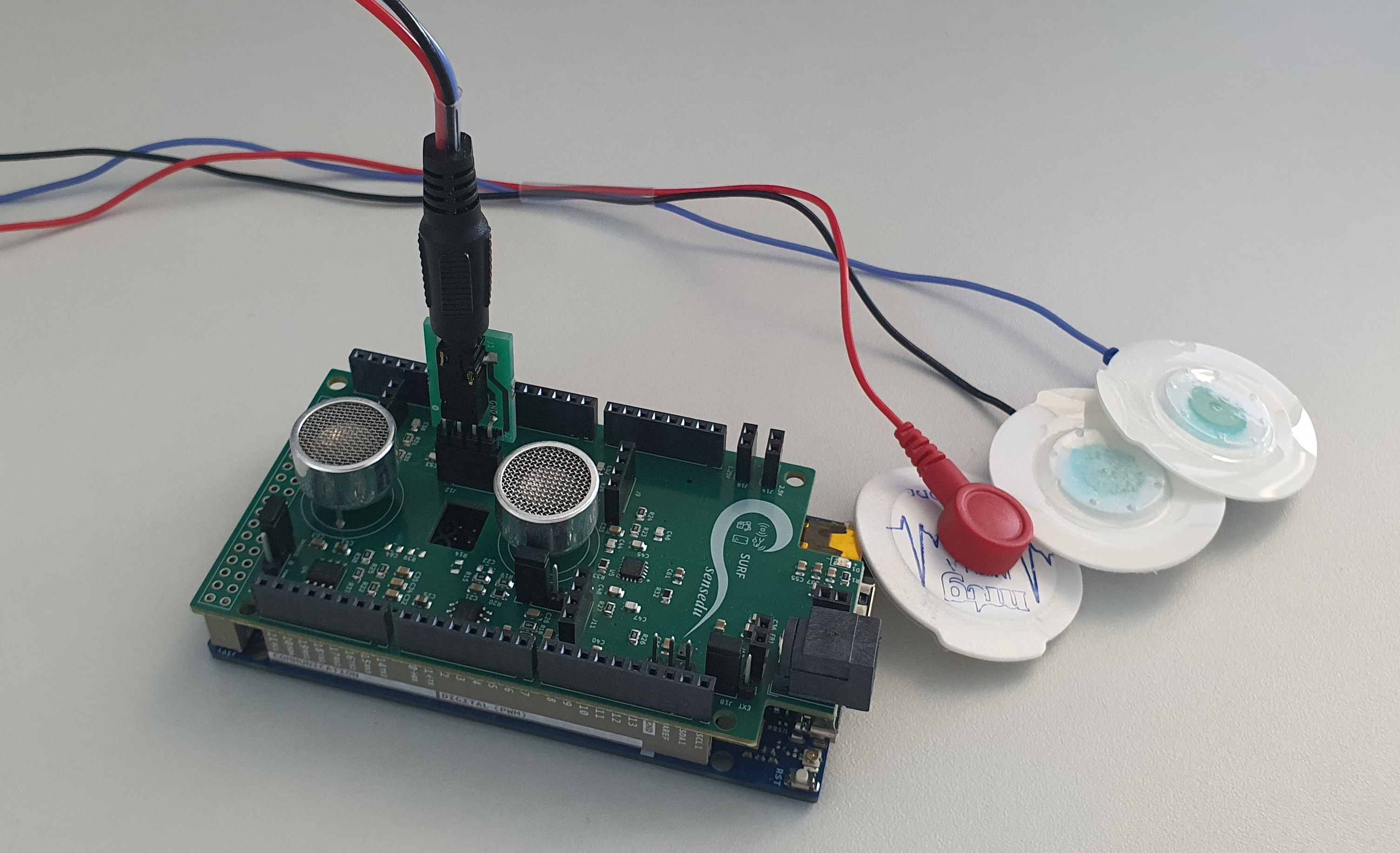
Electrode connection to SensEdu

Amplifier Circuit

The first stage after the input electrodes is signal amplification.

The idea is to detect a signal at two points, amplify the “difference”, and remove everything “common” between them. This way, the local EMG signal will be isolated and amplified. For that, we need a differential amplifier with a high Common Mode Rejection Ratio (CMRR), at least >\(90dB\).

Besides CMRR, an amplifier is also required to have a high input impedance. The impedance of the electrode-skin interface can vary from several thousand ohms to several megohms for dry skin. In order to prevent attenuation and distortion of the detected signal due to the effects of input loading, the input impedance of the differential amplifier should be as large as possible.

A differential amplifier with input buffer amplifiers, which features very high CMRR and input impedance, is called an Instrumentation Amplifier. SensEdu is equipped with this type of amplifiers, specifically the x2 dual-channel AD8222, making the platform suitable for bio-signal measurements.

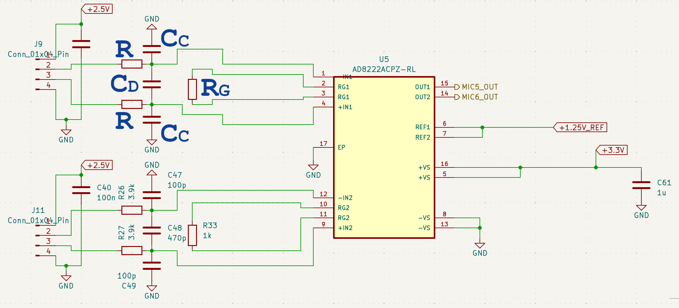
Amplification Circuit

Gain is set by \(R_G\) resistor, using the following formula:

\[G = 1 + \frac{49.4kΩ}{R_G} = 1 + \frac{49.4kΩ}{1kΩ} = 50.4\]

To avoid high frequency rectification and thus signal distortions, additional filtering is applied at the input. The filter limits the input signal bandwidth according to the following relationships:

\[{f_c}_{DIFF} = \frac{1}{2\pi × R(2C_D + C_C)} = \frac{1}{2\pi × 3.9kΩ(2×470pF + 100pF)} = 37.7\mathrm{kHz}\] \[{f_c}_{CM} = \frac{1}{2\pi × R × C_C} = \frac{1}{2\pi × 3.9kΩ × 100pF} = 392.2\mathrm{kHz}\]

Mismatch between \(R × C_C\) at the positive and negative inputs degrades the CMRR of the AD8222. By using a value for \(C_D\) that is ~10× larger than \(C_C\), the effect of the mismatch is reduced and performance is improved.

We used the default \({f_c}_{DIFF}\) and \({f_c}_{CM}\) cutoff frequencies for all projects, which were originally selected to suit the ultrasonic use case. Additional optimization is possible by reducing these cutoff frequencies to align with the working range of EMG signals (up to ~\(500\mathrm{Hz}\)). It could result in improved signal quality and reduced post‐processing requirements.

To write Arduino scripts for EMG signal acquisition, it is crucial to understand how the amplifier I/O is wired. Specifically, the following details:

• Which input header is connected to each amplifier channel
• Which amplifier output corresponds to which ADC channel on the MCU

All these details are available in the SensEdu schematics and ADC mapping table. For convenience, the table below provides a summary of the relevant connections:

Input Header	Amplifier Channel	Output Arduino Pin	Output STM32 Pin	Available ADCs
J9	U5 CH1	A0	PC4	ADC1 & ADC2
J11	U5 CH2	A2	PB0	ADC1 & ADC2
J12	U6 CH1	A11	PA0_C	ADC1 & ADC2
J20	U6 CH2	A7	PA0	ADC1

Data Acquisition

The next step is to write and configure the Arduino sketch responsible for data acquisition. This involves configuring ADC parameters, such as sampling rate, buffer size, memory mode, etc.

For EMG, a sampling rate of about \(1.5\mathrm{kHz}\) is usually sufficient. However, to improve the quality of future digital post-processing, this project uses a high oversampling rate of \(f_s = 25.6\mathrm{kHz}\). Each channel uses a buffer of \(N_s = 1024 \ \mathrm{samples}\). ADC is configured with DMA to minimize CPU load and maximize performance. The ideal theoretical duration of one complete measurement cycle is given as:

\[d_{meas, \ ideal} = \frac{N_s}{f_s} = \frac{1024 \ \mathrm{samples}}{25.6\mathrm{kHz}} = 40\mathrm{ms}\]

The measurement duration is independent of the number of selected channels. ADC is designed to maintain its sampling frequency per channel.

In practice, the actual \(d_{meas}\) varies between approximately \(46-51\mathrm{ms}\) due to delays from data transmission, wasted CPU cycles, ADC conversion rate fluctuations, and other factors. In the end, it results in a practical measurement rate at around \(20\) measurements per second. If this performance is not satisfactory, revisit the adjustment of ADC parameters.

Keeping selected parameters in mind, the ADC can be configured using SensEdu Library. The configuration follows similar structure to the Read_ADC_3CH_DMA example. Below is a minimal code example, focusing on the essential lines.

ADC_TypeDef* adc = ADC1;
const uint16_t channel_count = 4;
uint8_t adc_pins[channel_count] = {A0, A2, A11, A7};
const uint16_t sampling_rate = 25600;

const uint16_t mem_size = 16 * channel_count * 64; // must be a multiple of 16
__attribute__((aligned(__SCB_DCACHE_LINE_SIZE))) uint16_t emg_data[mem_size];

SensEdu_ADC_Settings adc_settings = {
    .adc = adc,
    .pins = adc_pins,
    .pin_num = channel_count,

    .conv_mode = SENSEDU_ADC_MODE_CONT_TIM_TRIGGERED,
    .sampling_freq = sampling_rate,
    
    .dma_mode = SENSEDU_ADC_DMA_CONNECT,
    .mem_address = (uint16_t*)emg_data,
    .mem_size = mem_size
};

Once the parameters are selected, the ADC must be initialized, enabled, and started.

void setup() {
    Serial.begin(115200);
    SensEdu_ADC_Init(&adc_settings);
    SensEdu_ADC_Enable(adc);
    SensEdu_ADC_Start(adc);
}

In the main loop, ensure that ADC completed its conversions and that DMA transferred the data. Transfer the data to PC, and restart the ADC again.

void loop() {
    while(!SensEdu_ADC_GetTransferStatus(adc));
    transfer_serial_data(&(emg_data[0]), mem_size, 64);

    SensEdu_ADC_ClearTransferStatus(adc);
    SensEdu_ADC_Start(adc);
}

The final expanded sketch is available at /projects/EMG-BioInputs/EMG-BioInputs.ino. It differs from above snippets in that it sends all configuration data to MATLAB during initialization. Additionally, the measurement process is triggered by MATLAB at each iteration to simplify data synchronization.

Data Transfer

Arduino GIGA R1 doesn’t use a typical UART interface for serial communication. Instead, it uses USB communication abstracted to behave like a serial link. This implementation makes the connection baud rate independent, meaning the number in Serial.begin() has no effect on the actual transfer speed. For further details on the USB implementation, refer to Figure 793 (Page 2747) of STM32H747 Reference Manual (OTG_FS) and the USB0 in the Arduino GIGA R1 Schematics.

To maximize the USB efficiency, data should be arranged and transferred in chunks. Based on tests in this repository, the optimal chunk size is 64 bytes, as specified in the OTG_FS section of the reference manual. Below is an example of how to implement chunked data transfer via USB.

// chunk_size in bytes, for OTG_FS "64" is passed
void transfer_serial_data(uint16_t* buf, const uint16_t buf_size, const uint16_t chunk_size) {
    for (uint16_t i = 0; i < (buf_size*2); i += chunk_size) {
        uint16_t cur_chunk_size = ((buf_size*2) - i < chunk_size) ? (buf_size*2 - i) : chunk_size;
        Serial.write((const uint8_t *) buf + i, cur_chunk_size);
    }
}

Alternatively, WiFi can be used for data transfer by implementing a method similar to the Basic_UltraSound_WiFi example.

Signal Processing

EMG post-processing was made in MATLAB. You can find the main block diagram below. The main components of filtering contains of storing the data in a longer buffer, applying filtering, enveloping and making a decision based on the final processed data: either the button on the keyboartd is presed, hold or released.

[picture: block diagram]

Problematic ADC Readings

First, let’s discuss the incoming RAW data to MATLAB. There was noticed a weird behaviour with the first couple of samples at each measurement cycle. They always abnormally high and after 5-10 samples stabilized around expected values.

[picture: weired samples]

It is not certain what exactly causes this behaviour, most probably is high input capacitance to ADC due to using the electrodes and all this bio setup.

To fix it fast, script just removes the first 8 samples from each measurement cycle, using only stable ADC data, keep that in mind while calculating the sizes for next steps.

The Buffer

After triggering the measurement cycle which lasts for \(d_{meas, ideal} = 40\mathrm{ms}\), the incoming data is stored in a buffer that contains the whole 1 second of these measurement cycles. Works like FIFO, the oldest measurement is out, the whole buffer shifts to the left and the freed up space is taken by the new one.

The buffer size is calculated based on \(d_{meas, ideal}\) which means that actual buffer contains data for a bit longer period than calculated.

Processing on this longer buffer helps multiple cycles of low-frequency components being captured and properly filtered out which improves filter’s ability to attenuate noise and artifact and preservation of desired signal components.

A longer history allows low-pass filters (used in envelope detection) to smooth the rectified signal over a larger time frame, resulting in a more robust and stable envelope.

For example, a 5Hz low-pass filter requires at least 200ms of data for one full cycle. With a 1-second history, the envelope will be less sensitive to short-term fluctuations or noise.

Use a 1-second buffer for filtering and envelope detection, but process overlapping chunks (e.g., update every 40ms). This ensures that decisions are updated frequently without sacrificing the filtering accuracy of the longer window.

There is a logic that doesn’t start the plotting or decision making before the whole buffer is filled when you start the program.

FIR Filter

Rectification

Envelope

Decision Block

MATLAB magic

1. full wave rectification

ull wave rectification In a first step, all negative amplitudes are converted to positive amplitudes; the negative spikes are “moved up” to positive or reflected by the baseline (Fig. 37). Besides easier reading, the main effect is that standard amplitude parameters like mean, peak/max value and area can be applied to the curve (raw EMG has a mean value of zero).

1. envelope

1. envelope ver2

Press problems

Capacitive input

ignore some of the first samples for ADC stabilization

https://devzone.nordicsemi.com/f/nordic-q-a/80796/adc—first-read-is-always-wrong/336435

Testing

Motor point regions Due to increased signal instability some researchers recommend not to place electrodes over motor point regions (area with high density of motor endplates) of the muscle. When using electrode sizes as recommended above, in many cases it cannot be avoided that one electrode comes near a motor point region. Motor points can be detected by low frequency stimulus power generators producing right angled impulses.

Most of the important limb and trunk muscles can be measured by surface electrodes (right side muscles in Fig. 26a/26b). Deeper, smaller or overlaid muscles need a fine wire application to be safely or selectively detected. The muscle maps show a selection of muscles that typically have been investigated in kinesiological studies. The two yellow dots of the surface muscles indicate the orientation of the electrode pair in ratio to the muscle fiber direction (proposals compiled from 1, 4, 10 and SENIAM).

At least one neutral reference electrode per subject needs to be positioned. Typically an electrically unaffected but nearby area is selected, such as joints, bony area, frontal head, processus spinosus, christa iliaca, tibia bone etc

Due to differential amplification against any reference, the latest amplifier technology (NORAXON active systems) needs no special area but only a location nearby the first electrode site.

RULES:

Showcase

WASD Dark Souls for 4 channels?

Possible improvements

EMG recording should not use any hardware filters (e.g. notch filters), except the amplifier bandpass (10 – 500 Hz) filters that are needed to avoid anti-aliasing effects within sampling.

Especially any type of notch filter (to e.g. cancel out 50 or 60 Hz noise) is not accepted because it destroys too much EMG signal power. Biofeedback units working with heavily preprocessed signals should not be used for scientific studies.

Implement filtering in hardware, you can extend SensEdu with another custom shield which will make half of current signal processing unnecessary greatly reducing latency and required computations. In addition, use right leg drive to decrease noise and offset.

Appendix: data recordings for improvements

Good study on perfect high pass value

https://www.bu.edu/nmrc/files/2010/06/103.pdf

Good Resources:

• https://www.nature.com/articles/s41597-022-01484-2
• https://abdominalkey.com/electromyography/
• https://hermanwallace.com/download/The_ABC_of_EMG_by_Peter_Konrad.pdf

Sources:

• https://youtu.be/_k6QINRcdV4?si=rnil7B-ZlqmRCGSN
• https://youtu.be/ApaPlKPb4ek?si=rHncr0b2XipqN83i